Models with Multiple Predictors

Code

library(tidyverse)

Horse hearts

We will use the horses’ hearts dataset. There are seven variables represented as columns. They comprise six ultrasound measurements and the weights of 46 horses’ hearts, specifically:

INNERSYS : Inner-wall ultrasound measurement in systole phase.
INNERDIA : Inner-wall ultrasound measurement in diastole phase.
OUTERSYS : Outer-wall ultrasound measurement in systole phase.
OUTERDIA : Outer-wall ultrasound measurement in diastole phase.
EXTSYS : Exterior ultrasound measurement in systole phase.
EXTDIA : Exterior ultrasound measurement in diastole phase.
WEIGHT : Weight in kilograms.

We will build a multiple regression model to predict the weights of hearts using the six ultrasound measurements.

Load data

Code

hh <- read_csv("../data/horsehearts.csv")

Pairs plot

Code

library(GGally)

ggpairs(hh)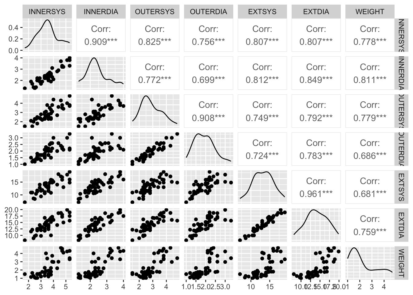

This plot reveals some very high correlation amongst predictors, particularly (not surprisingly) between the same measurements taken in the different phases (diastolic and systolic). Thus, multicollinearity is likely to be a problem when fitting a multiple regression model. The challenge will be choose the subset of variables that provides the best model fit.

`lm` output

Let’s start by fitting the full model with all of the available predictor variables.

The formula WEIGHT ~ . fits a model with WEIGHT as the response variable and all other variables in the data frame as predictor variables.

Code

mf <- lm(WEIGHT ~ . , data = hh)

summary(mf)


Call:
lm(formula = WEIGHT ~ ., data = hh)

Residuals:
     Min       1Q   Median       3Q      Max 
-0.92909 -0.30000 -0.00898  0.29517  1.38196 

Coefficients:
             Estimate Std. Error t value Pr(>|t|)    
(Intercept) -2.246014   0.427517  -5.254 6.00e-06 ***
...1         0.030946   0.007098   4.360 9.58e-05 ***
INNERSYS     0.487587   0.261681   1.863   0.0702 .  
INNERDIA     0.145040   0.338119   0.429   0.6704    
OUTERSYS     0.219805   0.294408   0.747   0.4599    
OUTERDIA    -0.302799   0.377546  -0.802   0.4275    
EXTSYS      -0.109803   0.119516  -0.919   0.3640    
EXTDIA       0.217405   0.125150   1.737   0.0905 .  
---
Signif. codes:  0 '***' 0.001 '**' 0.01 '*' 0.05 '.' 0.1 ' ' 1

Residual standard error: 0.4968 on 38 degrees of freedom
Multiple R-squared:  0.835, Adjusted R-squared:  0.8047 
F-statistic: 27.48 on 7 and 38 DF,  p-value: 5.195e-13

Interpreting summary.lm output

There is a lot of information in the above summary output to process. Let’s break it down.

The Call part shows us the command we used to produce the model.
The Residuals part gives us a five-number summary of the residuals.
The Coefficients table provides the estimates of the model parameters. Specifically, the Estimate column gives us the estimates of the \(\beta\)-coefficients, which can be used to reconstruct the predictive formula. Here, that formula is:

\[\hat y = -1.6311 + 0.2321 × INNERSYS + 0.5195 × INNERDIA + ... + 0.3387 × EXTDIA\]

The Std. Error column gives the standard error for the estimates of the coefficients. That is, the expected average deviation of the estimator of the coefficient (\(b\) or \(\hat \beta\)) from the true population parameter (\(\beta\)). If we were to take many samples (of size \(n\)) from this population, a coefficient’s standard error represents how much the estimate is expected to vary (due to sampling variation).

The t value is the estimate divided by its standard error, which can be used to test whether the effect of that variable is statistically different from zero. The p-value for this test is provided in the next column, headed Pr(>|t|). If the p-value is low, the observed coefficient estimate is unlikely to have resulted by chance due to sampling variation if the null hypothesis (\(H_0 : \beta = 0\)) is true. Asterisks indicate significant results, as coded by the Signif. codes: given below the table.
The final three lines give results for the entire model.

The final three lines give results for the entire model.

The Residual standard error is an estimate of the standard deviation of the residuals, i.e. the average absolute difference between the predicted values and the actual values. When estimating the weight of horse’s hearts using this model, we would expect to, on average, be wrong by 0.6 kg. The degrees of freedom here are the residual degrees of freedom—the number of independent pieces of information with which the residual standard error was estimated.

Next, we have the Multiple R-squared, which is the proportion of the total variation in y that is explained by the model. Here, 75% of the variation is explained. The Adjusted R-squared is adjusted for the number of variables included in the model (see lecture slides). It cannot be interpreted in same way as the unadjusted \(R^2\) can, but it can be used to compare models.

Finally, an F-statistic, associated degrees of freedom (DF) , and p-value are provided. This tests whether the model explains a significant proportion of the total variation in y. This can be thought of as testing whether any of the \(\beta\) coefficients in model are non-zero. Here, the p-value is very small so we reject the null hypothesis that all of the \(\beta\) coefficients in model are zero.

Variance Inflation Factor

We mentioned earlier that we were concerned with multicollinearity—correlation among the predictors. A consequence of multicollinearity is that it increases the uncertainty in the estimates of the coefficients—the standard errors of the coefficients are inflated. We can quantify this effect, for each coefficient, with the Variance Inflation Factor (VIF). This is given by the function car::vif()¹.

Code

car::vif(mf)

     ...1  INNERSYS  INNERDIA  OUTERSYS  OUTERDIA    EXTSYS    EXTDIA 
 1.655390  9.236266  9.196188  9.031392  6.826111 18.501906 23.139222

According to a rule of thumb, a VIF > 5 is cause for some concern. A VIF > 10 is definitely problematic. So, we have a problem here.

The above VIF values pertain to variances. I find it more intuitive to discuss the square root of the VIF because they relate to the standard errors.

Code

sqrt(car::vif(mf))

    ...1 INNERSYS INNERDIA OUTERSYS OUTERDIA   EXTSYS   EXTDIA 
1.286619 3.039123 3.032522 3.005227 2.612683 4.301384 4.810325

These \(\sqrt{}\)VIF values can be interpreted in the following way: the standard error for the effect of INNERSYS is around three times larger because of the presence of the other (correlated) variables in the model. The VIF is greatest for EXTDIA, which is consistent with this variable seeming to have the highest correlations with the other predictors.

Model selection

Statisticians use the term “parsimonious” to describe a model that contains no more predictors than necessary to adequately model the data—a model that has the right balance of complexity.

Let’s run a stepwise model selection process to try to find a more parsimonious model than the full model created above. The criterion we will use to assess the quality of the models is Akaike Information Criterion (AIC). Lower AIC values (i.e. closer to \(-\infty\)) are better.

We will undertake a stepwise process in individual steps, using the drop1() function.

Code

drop1(mf)

Single term deletions

Model:
WEIGHT ~ ...1 + INNERSYS + INNERDIA + OUTERSYS + OUTERDIA + EXTSYS + 
    EXTDIA
         Df Sum of Sq     RSS     AIC
<none>                 9.3771 -57.157
...1      1    4.6903 14.0675 -40.500
INNERSYS  1    0.8567 10.2339 -55.135
INNERDIA  1    0.0454  9.4226 -58.935
OUTERSYS  1    0.1376  9.5147 -58.487
OUTERDIA  1    0.1587  9.5359 -58.385
EXTSYS    1    0.2083  9.5854 -58.146
EXTDIA    1    0.7447 10.1218 -55.642

We have taken the full model (all predictors included) and asked what the AIC values² would be obtained if we dropped each one of the predictors (or none). The lowest AIC score is for the model with INNERSYS removed… so let’s remove it and then use drop1() again.

Code

m2 <- update(mf, ~ . - INNERSYS)
drop1(m2)

Single term deletions

Model:
WEIGHT ~ ...1 + INNERDIA + OUTERSYS + OUTERDIA + EXTSYS + EXTDIA
         Df Sum of Sq    RSS     AIC
<none>                10.234 -55.135
...1      1    4.0379 14.272 -41.836
INNERDIA  1    1.7508 11.985 -49.871
OUTERSYS  1    0.4701 10.704 -55.069
OUTERDIA  1    0.0910 10.325 -56.728
EXTSYS    1    0.0442 10.278 -56.937
EXTDIA    1    0.3723 10.606 -55.491

Now we remove OUTERDIA and repeat.

Code

m3 <- update(m2, ~ . - OUTERDIA)
drop1(m3)

Single term deletions

Model:
WEIGHT ~ ...1 + INNERDIA + OUTERSYS + EXTSYS + EXTDIA
         Df Sum of Sq    RSS     AIC
<none>                10.325 -56.728
...1      1    4.4141 14.739 -42.355
INNERDIA  1    1.9579 12.283 -50.740
OUTERSYS  1    0.5073 10.832 -56.522
EXTSYS    1    0.0208 10.346 -58.635
EXTDIA    1    0.2912 10.616 -57.448

This time, the best model is that with none removed, so the model selection process stops there. Note that this whole process could have been done in a single line of code.

Code

mstep <- step(mf)

Start:  AIC=-57.16
WEIGHT ~ ...1 + INNERSYS + INNERDIA + OUTERSYS + OUTERDIA + EXTSYS + 
    EXTDIA

           Df Sum of Sq     RSS     AIC
- INNERDIA  1    0.0454  9.4226 -58.935
- OUTERSYS  1    0.1376  9.5147 -58.487
- OUTERDIA  1    0.1587  9.5359 -58.385
- EXTSYS    1    0.2083  9.5854 -58.146
<none>                   9.3771 -57.157
- EXTDIA    1    0.7447 10.1218 -55.642
- INNERSYS  1    0.8567 10.2339 -55.135
- ...1      1    4.6903 14.0675 -40.500

Step:  AIC=-58.93
WEIGHT ~ ...1 + INNERSYS + OUTERSYS + OUTERDIA + EXTSYS + EXTDIA

           Df Sum of Sq     RSS     AIC
- OUTERSYS  1    0.1311  9.5537 -60.299
- OUTERDIA  1    0.2021  9.6246 -59.959
- EXTSYS    1    0.2544  9.6769 -59.709
<none>                   9.4226 -58.935
- EXTDIA    1    1.0850 10.5076 -55.921
- INNERSYS  1    2.5621 11.9847 -49.871
- ...1      1    5.2676 14.6902 -40.507

Step:  AIC=-60.3
WEIGHT ~ ...1 + INNERSYS + OUTERDIA + EXTSYS + EXTDIA

           Df Sum of Sq     RSS     AIC
- OUTERDIA  1    0.0739  9.6276 -61.945
- EXTSYS    1    0.2119  9.7655 -61.290
<none>                   9.5537 -60.299
- EXTDIA    1    1.0287 10.5824 -57.595
- INNERSYS  1    3.6497 13.2034 -47.416
- ...1      1    6.9595 16.5132 -37.126

Step:  AIC=-61.94
WEIGHT ~ ...1 + INNERSYS + EXTSYS + EXTDIA

           Df Sum of Sq     RSS     AIC
- EXTSYS    1    0.1741  9.8017 -63.120
<none>                   9.6276 -61.945
- EXTDIA    1    0.9636 10.5912 -59.557
- INNERSYS  1    3.7894 13.4170 -48.677
- ...1      1    6.8859 16.5134 -39.126

Step:  AIC=-63.12
WEIGHT ~ ...1 + INNERSYS + EXTDIA

           Df Sum of Sq     RSS     AIC
<none>                   9.8017 -63.120
- EXTDIA    1    2.1043 11.9060 -56.174
- INNERSYS  1    3.6186 13.4203 -50.666
- ...1      1    9.8369 19.6386 -33.153

When you run this, the whole three-step process we executed above will print onscreen and the object mstep represents the stepwise-selected model.

Let’s examine the stepwise model.

Code

summary(mstep)


Call:
lm(formula = WEIGHT ~ ...1 + INNERSYS + EXTDIA, data = hh)

Residuals:
     Min       1Q   Median       3Q      Max 
-0.89894 -0.28511 -0.03404  0.30224  1.16660 

Coefficients:
             Estimate Std. Error t value Pr(>|t|)    
(Intercept) -2.418691   0.368870  -6.557 6.27e-08 ***
...1         0.035665   0.005493   6.492 7.77e-08 ***
INNERSYS     0.559216   0.142016   3.938 0.000304 ***
EXTDIA       0.128883   0.042921   3.003 0.004492 ** 
---
Signif. codes:  0 '***' 0.001 '**' 0.01 '*' 0.05 '.' 0.1 ' ' 1

Residual standard error: 0.4831 on 42 degrees of freedom
Multiple R-squared:  0.8276,    Adjusted R-squared:  0.8153 
F-statistic: 67.19 on 3 and 42 DF,  p-value: 4.476e-16

We still have two variables that are very highly correlated: EXTSYS and EXTDIA. Let’s see if this correlation is problematic, according to the VIF criterion.

Code

car::vif(mstep)

    ...1 INNERSYS   EXTDIA 
1.048398 2.876504 2.877824

With VIF scores for these two variables still well above 5, this is certainly a problem. This illustrates an important point: you must not naively accept a model which results from a stepwise selection process. Always scrutinise a model before accepting it.

We will force a step where we drop either EXTSYS or EXTDIA.

Code

drop1(mstep)

Single term deletions

Model:
WEIGHT ~ ...1 + INNERSYS + EXTDIA
         Df Sum of Sq     RSS     AIC
<none>                 9.8017 -63.120
...1      1    9.8369 19.6386 -33.153
INNERSYS  1    3.6186 13.4203 -50.666
EXTDIA    1    2.1043 11.9060 -56.174

Code

mstep2 <- update(mstep,  ~ . - EXTDIA)

Now, let’s try another step.

Code

drop1(mstep2)

Single term deletions

Model:
WEIGHT ~ ...1 + INNERSYS
         Df Sum of Sq    RSS     AIC
<none>                11.906 -56.174
...1      1    10.535 22.441 -29.017
INNERSYS  1    25.822 37.728  -5.119

It seems that the model with EXTSYS removed, leaving only INNERDIA and OUTERSYS, is actually preferable. Once the latter two variables are included, EXTSYS does not add any strength to the model. Let’s make this model and check for further removals, and our VIFs.

Code

mstep3 <- update(mstep2, ~ . - EXTSYS)
drop1(mstep3)

Single term deletions

Model:
WEIGHT ~ ...1 + INNERSYS
         Df Sum of Sq    RSS     AIC
<none>                11.906 -56.174
...1      1    10.535 22.441 -29.017
INNERSYS  1    25.822 37.728  -5.119

Code

car::vif(mstep3)

    ...1 INNERSYS 
1.043276 1.043276

It seems that this model cannot be improved by dropping any further variables. The variables INNERDIA and OUTERSYS, though correlated (r = 0.77), do not exert undue influence on each other in the model.

To summarise, let’s see the AIC scores for all the models we’ve made so far.

Code

AIC(mf, m2, m3, mstep, mstep2, mstep3)

       df      AIC
mf      9 75.38552
m2      8 77.40723
m3      7 75.81462
mstep   5 69.42241
mstep2  4 76.36871
mstep3  4 76.36871

All of these models have very similar AIC. Statisticians say that AIC scores within, say, 3 points can be considered equivalent, and so often we take the approach of choosing the simplest model (i.e. that with the fewest predictors) of all those within 3 AIC points of the lowest score. In some fields it is common to report all models within 10 AIC points or produce an ensemble model bases on AIC weight (not covered in this course). So, while the mstep3 model isn’t the absolute lowest, it is the simplest model from a bunch of models with roughly equivalent AIC scores. Also, it is a good choice because it doesn’t have the problems with severe multicollinearity found in the other models.

Don’t worry about the fact that the two functions drop1() and AIC() give different scores. Remember the AIC is a tool for comparing models—the actual scores don’t matter. If you look at the difference in AIC scores between two models from the two functions, they are the same. It also should not be compared on models that have different data sources because it is unit less and only acts to compare the models in a specific set.

Difference between AIC scores for mstep2 and mstep3 from the drop1(mstep2) output:

Code

-40.395 - (-42.083)

[1] 1.688

And from the AIC(mf, m2, m3, mstep, mstep2, mstep3) output:

Code

92.14759 - 90.45888

[1] 1.68871

So now we can choose mstep3 and clean up.

Code

rm(mf, m2, m3, mstep, mstep2) # this code removes these variables

Let’s examine the summary for our chosen model.

Code

summary(mstep3)


Call:
lm(formula = WEIGHT ~ ...1 + INNERSYS, data = hh)

Residuals:
     Min       1Q   Median       3Q      Max 
-1.19304 -0.32850 -0.02243  0.37865  1.16895 

Coefficients:
             Estimate Std. Error t value Pr(>|t|)    
(Intercept) -1.837792   0.342098  -5.372 2.97e-06 ***
...1         0.036819   0.005969   6.168 2.08e-07 ***
INNERSYS     0.899656   0.093160   9.657 2.46e-12 ***
---
Signif. codes:  0 '***' 0.001 '**' 0.01 '*' 0.05 '.' 0.1 ' ' 1

Residual standard error: 0.5262 on 43 degrees of freedom
Multiple R-squared:  0.7906,    Adjusted R-squared:  0.7808 
F-statistic: 81.15 on 2 and 43 DF,  p-value: 2.529e-15

We are now explaining 72% of the variation in heart weights with two variables, as opposed to 75% of the variation with six variables in the original full model. Note also that, in the full model, INNERDIA was not significant and OUTERSYS was only weakly significant. In the smaller model, both these predictors were highly significant. Personally, I would definitely prefer the more parsimonious two-variable model, especially if it meant that I had only to take two, rather than six, ultrasound measurements on a thousand horses!

But we’re not done yet. We must use some diagnostic tools to examine whether our model meets the assumptions of linear regression before we can accept it.

Model diagnostics

Examine the usual four diagnostic plots.

Code

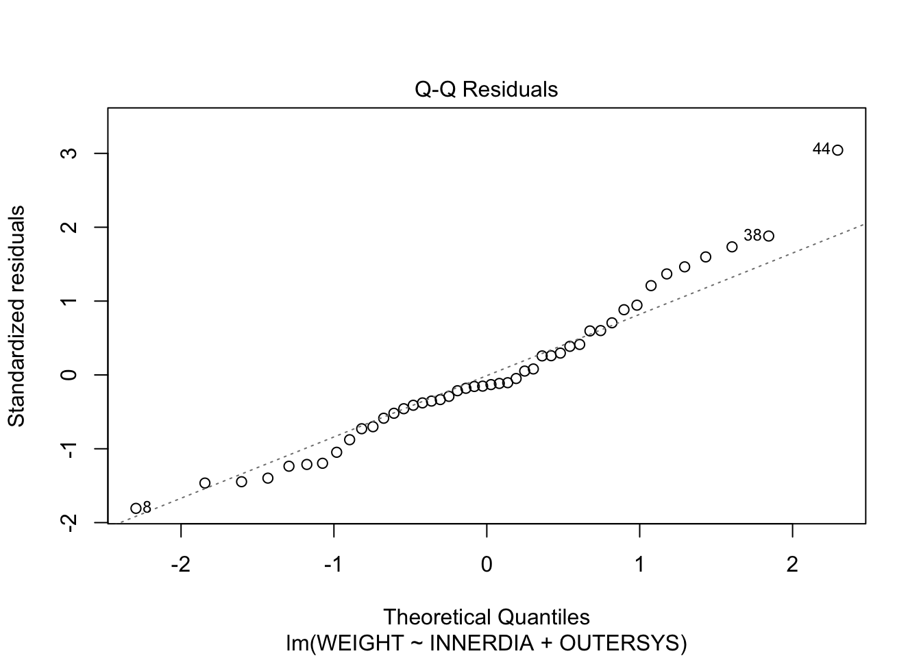
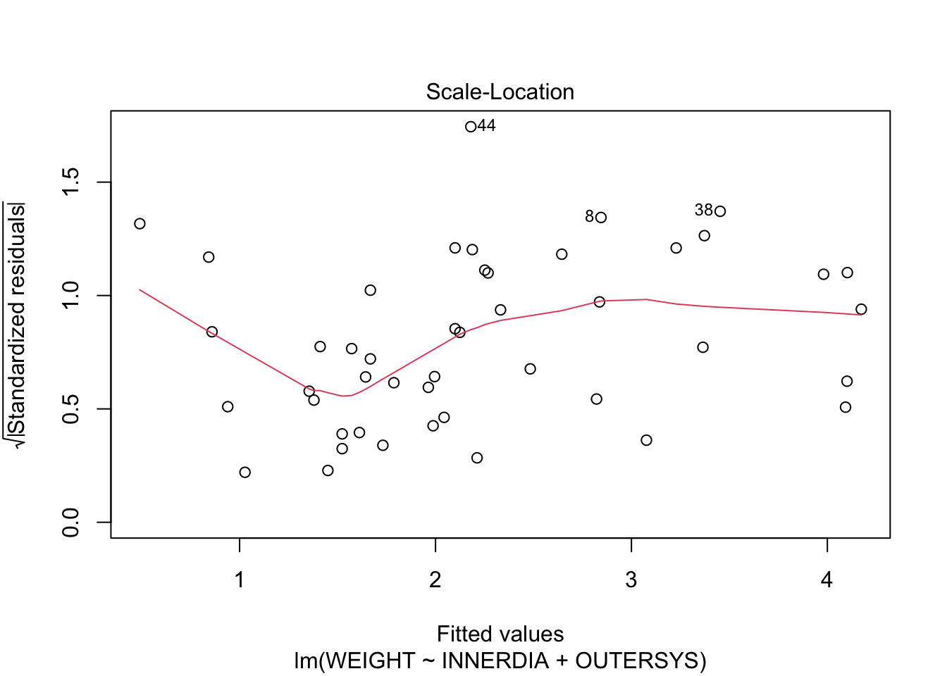
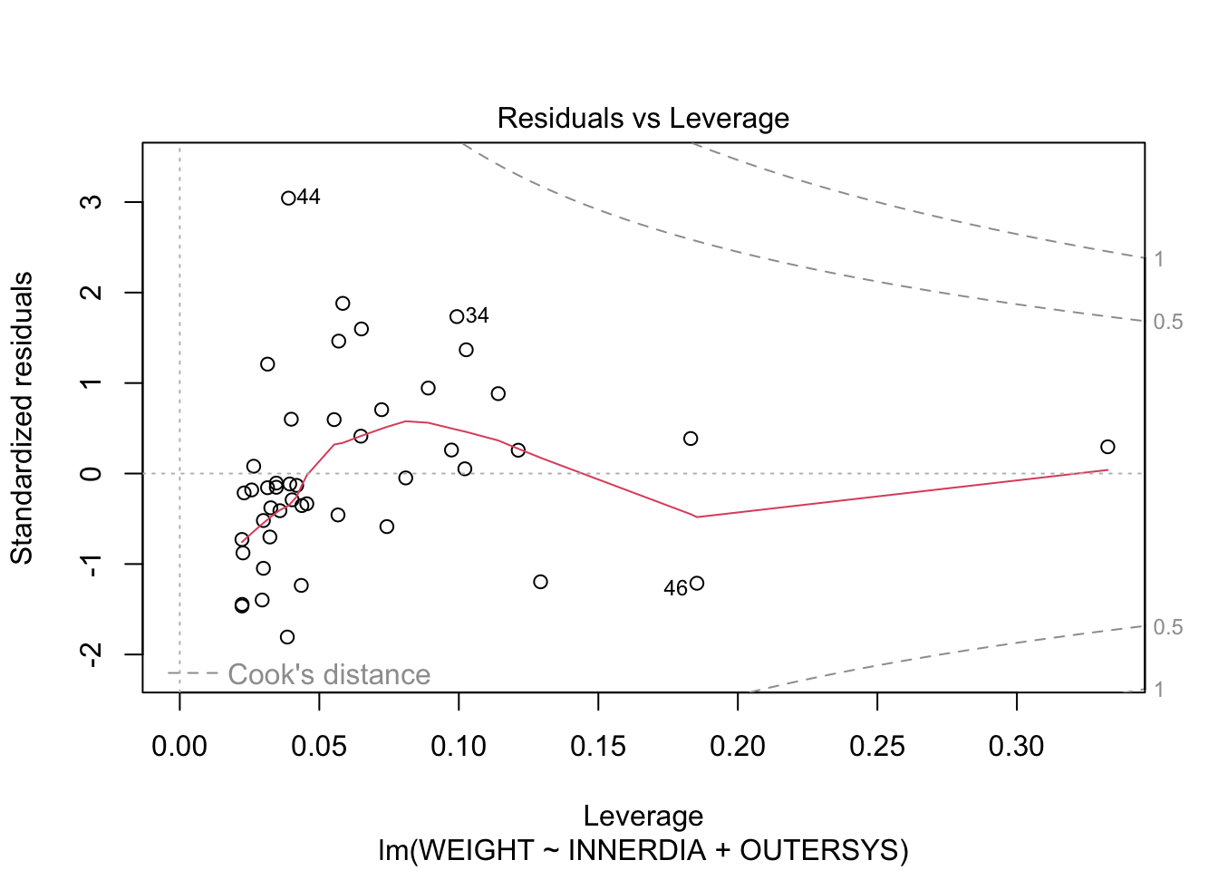
plot(mstep3)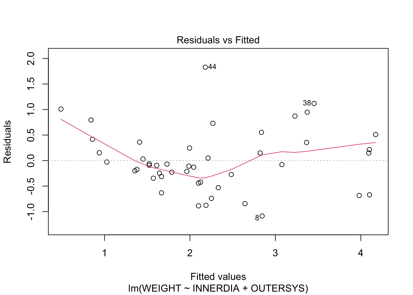

The Residuals-vs-Fitted plot shows a slight decreasing trend in the residuals at low fitted values, but it is only a few points. It might pay, though, to bear in mind that the model is likely to overestimate lower heart weights.

The normal Q-Q plot is not too worrying, although there are a few higher-than-expected residuals.

The Scale-Location plot shows no strong evidence of heteroscedasticity—the variance appears fairly constant across fitted values.

And, finally, there are no very large values of Cook’s distance or leverage.

There are many other diagnostic tools and graphs available, many in the car library, which we do not have time to go into here. If you’re interested, this website is a good place to start: http://www.statmethods.net/stats/rdiagnostics.html.

3D plots

Since there are three variables involved in this model, it might be useful to examine their relationship using 3D plots. We can include the 2D plane that represents our regression model on the plot, using the following code.

Code

library(scatterplot3d)

hh3d <- scatterplot3d(
  hh$INNERDIA, 
  hh$OUTERSYS, 
  hh$WEIGHT,
  type="h", 
  highlight.3d=T,
  pch=16
  )

hh3d$plane3d(mstep3)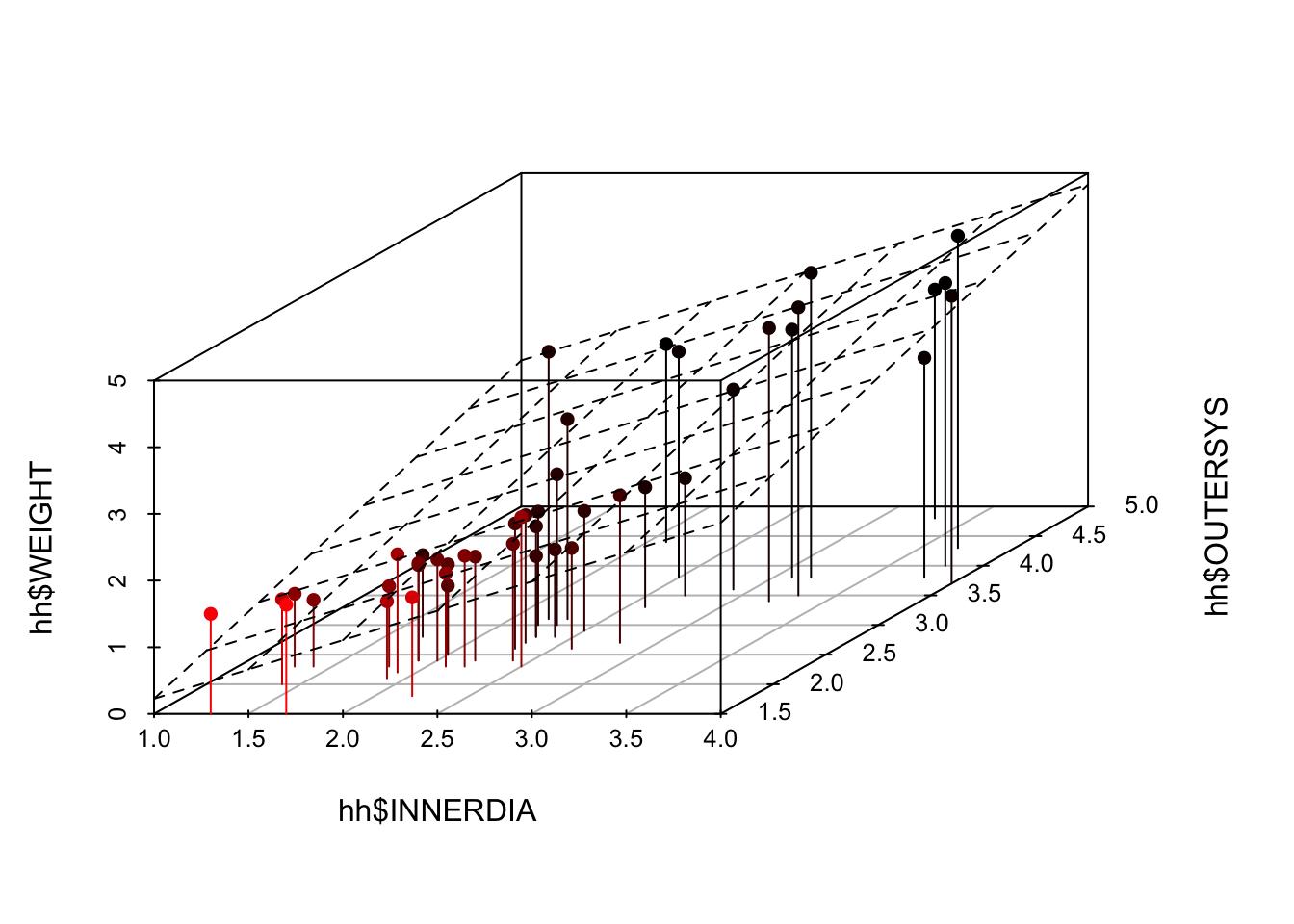

Finally, use plotly to create a dynamic 3D plot which you can rotate using your mouse. Don’t say I never treat you!

Code

library(plotly)

plot_ly(
  hh, 
  x = ~INNERDIA, 
  y = ~OUTERDIA, 
  z = ~WEIGHT
  ) |> 
  add_markers()

I do not recommend 3-D plots for print reports/publications. They are often best viewed interactively. Instead try using colors or bubbles for continuous third variables and shapes or facets for discrete third variables.

For example:

Code

hh |> ggplot(aes(y=OUTERDIA, x=INNERDIA, color=WEIGHT))+
  geom_point()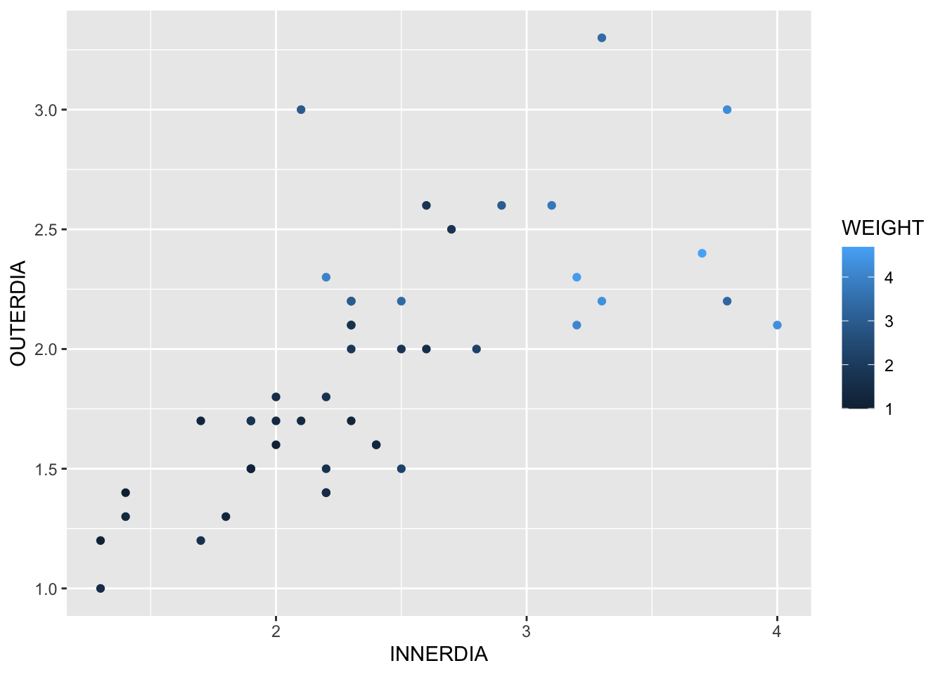

Dataset `Prestige`

We will continue to use dataset Prestige from the car R package.

Exercise 7.1

Obtain the matrix plot of the numerical variables education, income, women, and prestige.

Code

library(car)
library(GGally)
library(tidyverse)

Code

Prestige |> 
  select(prestige, education, income, women) |> 
  ggpairs(aes(colour=Prestige$type))

Obtain their correlation matrix.

Code

# Old style pairs plot
Prestige |> 
  select(prestige, education, income, women) |>
  pairs()

Code

Prestige |> 
  select(prestige, education, income, women) |>
  cor()

Fit a (full) multiple regression of prestige on education, income, & women.

Code

full.reg <- lm(prestige ~ education + income + women,
               data = Prestige)

Obtain the plots for residual diagnostics. Residual plots

Code

library(ggfortify)

autoplot(full.reg, 1:6)

Code

# Old style plots
plot(full.reg, 1) # the argument 1 can be changed up to 6

Code

# or just use
par(mfrow=c(2,2))
plot(full.reg)

Regression outputs

Code

summary(full.reg)


Call:
lm(formula = prestige ~ education + income + women, data = Prestige)

Residuals:
     Min       1Q   Median       3Q      Max 
-19.8246  -5.3332  -0.1364   5.1587  17.5045 

Coefficients:
              Estimate Std. Error t value Pr(>|t|)    
(Intercept) -6.7943342  3.2390886  -2.098   0.0385 *  
education    4.1866373  0.3887013  10.771  < 2e-16 ***
income       0.0013136  0.0002778   4.729 7.58e-06 ***
women       -0.0089052  0.0304071  -0.293   0.7702    
---
Signif. codes:  0 '***' 0.001 '**' 0.01 '*' 0.05 '.' 0.1 ' ' 1

Residual standard error: 7.846 on 98 degrees of freedom
Multiple R-squared:  0.7982,    Adjusted R-squared:  0.792 
F-statistic: 129.2 on 3 and 98 DF,  p-value: < 2.2e-16

Code

anova(full.reg)

Analysis of Variance Table

Response: prestige
          Df  Sum Sq Mean Sq  F value    Pr(>F)    
education  1 21608.4 21608.4 350.9741 < 2.2e-16 ***
income     1  2248.1  2248.1  36.5153 2.739e-08 ***
women      1     5.3     5.3   0.0858    0.7702    
Residuals 98  6033.6    61.6                       
---
Signif. codes:  0 '***' 0.001 '**' 0.01 '*' 0.05 '.' 0.1 ' ' 1

Code

extractAIC(full.reg)

[1]   4.0000 424.1724

Exercise 7.2

Perform stepwise regression analysis of prestige on education, income, & women.

Code

full.reg = lm(prestige ~ education + income + women,
              data = Prestige)

step(full.reg)

step(full.reg, direction="backward")

step(full.reg, direction="both")

The function update() is handy for making adjustments to a model. For example, see try the following codes:

Code

m1 = update(full.reg,  . ~ . - women)

summary(m1)

Note that . ~ . - women means that the model is fitted without the women variable.

Further options are available in leaps and HH packages (installation commands are given below).

install.packages("leaps", repos = "https://cran.r-project.org") install.packages("HH", repos = "https://cran.r-project.org")

Code

library(leaps)

model = regsubsets(prestige ~ education + income + women, 
                   data = Prestige)

library(HH)

summaryHH(model)

plot(summaryHH(model))

Exercise 7.3

Perform a polynomial regression of prestige on income.

Code

# Cubic fit
p.model <- lm(prestige ~ poly(income,3),
              data = Prestige)

summary(p.model)

extractAIC(p.model)

plot(p.model)

Code

autoplot(p.model)

Try it yourself

Use the river data from Assignment 1:

Code

riv <- read_csv("riverdat.csv")

Exercise 7.4

Make a scatterplot of all the raw values of Temperature (x-axis) and CHLA Mean (y-axis) for the Canterbury region only, with the points coloured by Catchment name. Fit a linear regression to the plot using geom_smooth.

Code

# your code goes here

Exercise 7.5

Fit a multiple linear regression for the Canterbury region only with the raw values of CHLA Mean as the response variable, Temperature and Dissolved oxygen as predictor variables. Produce a summary table and ANOVA table of your results.

Code

# your code goes here

Exercise 7.6

Make an indicator variable for the Waimakariri River catchment in Canterbury (0 = not in that catchment, 1 = in that catchment). Add this to your regression from exercise 7.5. Produce new tables and discuss your results.

Code

# your code goes here

More R code examples are here

Footnotes

The car::vif() notation calls the function vif() from within the package car. Alternatively, you can load the package into R with the command library(car). After doing this, all functions in the car package become available, so you can call the function directly as vif(), omitting the car::. Either way, you must have the package installed, of course!↩︎
Negative values of AIC, as seen here, are uncommon but are nothing to worry about. This occurs when the values of the response variable are small.↩︎

Horse hearts

Load data

Pairs plot

lm output

Variance Inflation Factor

Model selection

Model diagnostics

3D plots

Dataset Prestige

Exercise 7.1

Exercise 7.2

Exercise 7.3

Try it yourself

Exercise 7.4

Exercise 7.5

Exercise 7.6

Footnotes

`lm` output

Dataset `Prestige`