Chapter 0 R quarto and Tidy data

Installing `R` and RStudio

In this course, we will be using R https://www.r-project.org/, an open-source (i.e., free) software package for data analysis. This software is available for essentially all computing platforms (e.g. Windows, Linux, Unix, Mac) is maintained and developed by a huge community of users including many of the world’s foremost statisticians.

R is a programming language but you may not be required to do a lot of programming for your course work. R includes functions which enables us to perform a full range of statistical analyses.

For installing R software, please visit https://cran.stat.auckland.ac.nz/ and follow the instructions.

Note that the R software will be sitting in the background in RStudio and you will not be using the standalone version of R in this course.

RStudio https://www.rstudio.com/products/rstudio/ is an integrated development environment (IDE) for R. It includes a console and a sophisticated code editor. It also contains tools for plotting, history, debugging, and management of workspaces and projects. RStudio has many other features such as authoring HTML, PDF, Word Documents, and slide shows. In order to download RStudio (Desktop edition, open source), go to

https://www.rstudio.com/products/rstudio/download/

Download the installation file and run it. Note that RStudio must be installed after installing R.

R/RStudio can also be run on a cloud platform at https://rstudio.cloud/ after creating a free account. Be aware though that some of the packages covered in this course may not work in the cloud platform and there is a maximum amount of computing time. We do not recommend relying on the cloud platform for this course.

If you open RStudio, you will see something similar to the screen shot shown in Figure 1:

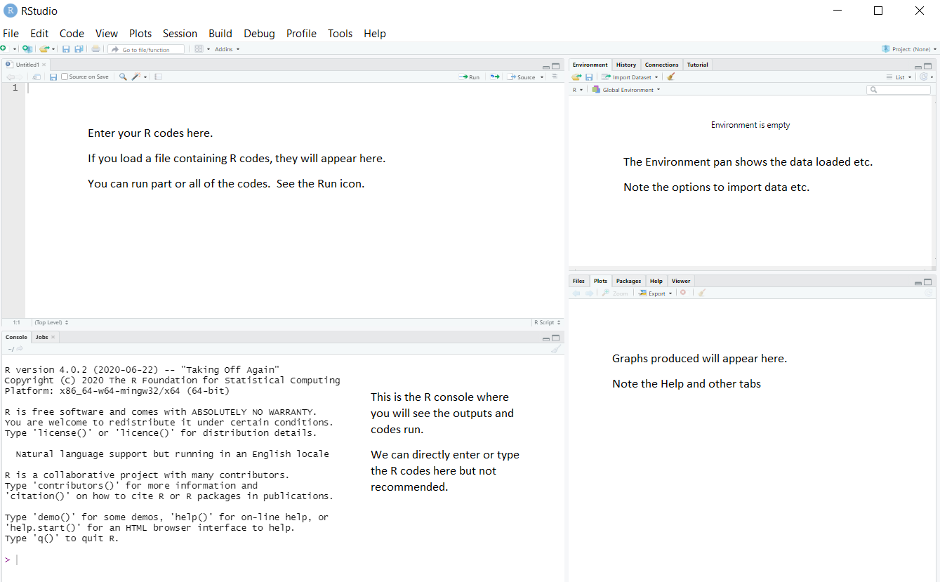
RStudio has many options, such as uploading files to a server, creating documents, etc. You will be using only a few of the options. You will not be using the menus such as Build, Debug, Profile at all in this course.

You can either type or copy and paste the R codes appearing in this section on to the R Script window and run them.

Quarto

This course will be using Quarto *.qmd files rather than raw *.R files. Heard of Rmarkdown? Well, Quarto is the successor to Rmarkdown. So, if you’re just starting to use R, then you should begin with Quarto rather than Rmarkdown, because most/all new development will be going into Quarto.

Here’s some information to get you started: https://quarto.org/docs/get-started/hello/rstudio.html.

And some other useful tips: https://r4ds.hadley.nz/quarto.

We will be using Quarto documents. You can open a blank one by clicking File > New File > Quarto Document.

You can then make your own document or copy code from the course website and paste it into your new Quarto file.

Including text and code

The one advantage of Quarto (and its predecessor R markdown) is being able to include general text along side code chunks.

You can insert a code chunk using the green button near the top right of your quarto document window.

Setting up a Quarto project

It is a good idea to get into the habit of using Quarto projects, rather than just R scripts. Here is a step-by-step guide to creating a project for your workshops. You don’t have to use projects, but they are very useful.

Open RStudio. (Optional: click on the little window symbol at the top and select “Console on Right”)

If you haven’t already, make a directory on your computer where you want to keep your code for this course.
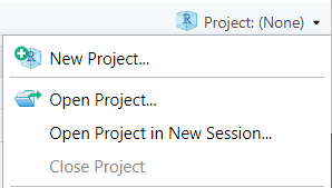
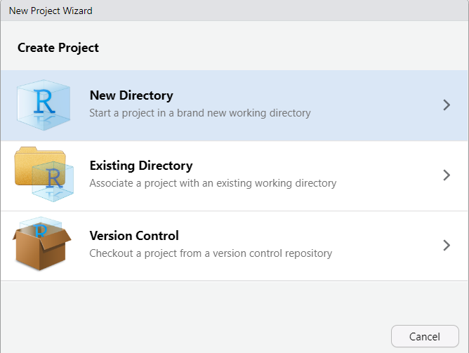
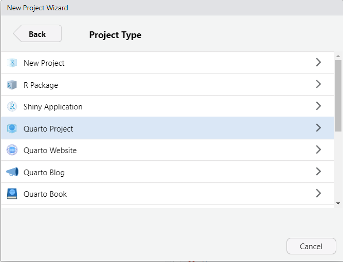
Make a new project. Select the “Project” button at the top-right of Rstudio, and select “New Project…”.

In the pop-up window:

Select “New Directory”

Select “Quarto Project”

Choose your directory via the “Browse”, and then give the project a name like “161250_workshops”

Finish by clicking on “Create Project”.

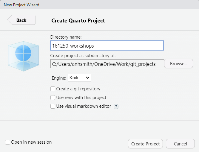
The project should now be created, and you’ll likely have an open *.qmd file (something like “161250_workshops.qmd”) in the top-right window of Rstudio. We want to make a *.qmd file for this workshop.

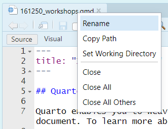
Right-click on the qmd tab and select “Rename”, and rename it “workshop2.qmd” or something similar. (Alternatively, just make a new file via the menus: File > New File > Quarto Document.)

Now you have a document for your Workshop work. You can:

Write headings with lines beginning with “#”.
Write text in the main part of the document.
Make a code chunk for your R code using Ctrl-Alt-i. Write R code in the code chunks.

Like so:

There are lots of tutorials online covering the basics of Quarto, and we’ll discuss them during our own workshops. Here are a couple for starters:

https://quarto.org/docs/get-started/hello/rstudio.html

https://www.youtube.com/watch?v=c654j7aQjcg

There are many advantages of Quarto projects. One is that you can put datasets into the project folder, and they’ll be easily accessible within your project, without having to worry about file paths.

You can easily open a recent past projects via the “Projects” button on the top-right of Rstudio.

This covers some introduces tidyverse and some functions we will be using in this course. This is not meant to be an exhaustive list and students are encourage to read R4 data science or other free tutorials online.

Definitions

Before we talk more about data it is useful to define some terms:

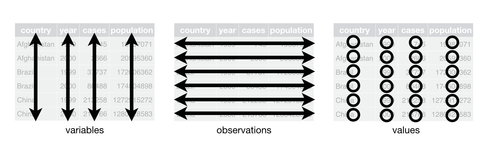
A variable is a quantity, quality, or property that you can measure.
A value is the state of a variable when you measure it. The value of a variable may change from measurement to measurement.
An observation is a set of measurements made under similar conditions (you usually make all of the measurements in an observation at the same time and on the same object). An observation will contain several values, each associated with a different variable. We’ll sometimes refer to an observation as a data point.
Tabular data is a set of values, each associated with a variable and an observation. Tabular data is tidy if each value is placed in its own “cell”, each variable in its own column, and each observation in its own row.

Introduction to the tidyverse

We will be largely using the tidyverse suite of packages for data organisation, summarising, and plotting; see https://www.tidyverse.org/.

Let’s load that package now:

Code

library(tidyverse)

Recommended reading to accompany this workshop is pages 1-11 of R for Data Science https://r4ds.hadley.nz/

Tidy data

There are three interrelated rules that make a dataset tidy:

Each variable is a column; each column is a variable.
Each observation is a row; each row is an observation.
Each value is a cell; each cell is a single value.

Why ensure that your data is tidy? There are two main advantages:

There’s a general advantage to picking one consistent way of storing data. If you have a consistent data structure, it’s easier to learn the tools that work with it because they have an underlying uniformity.
There’s a specific advantage to placing variables in columns because it allows R’s vectorized nature to shine. Most built-in R functions work with vectors of values.

dplyr, ggplot2, and all the other packages in the tidyverse are designed to work with tidy data.

Summarize data

Apply summary functions to columns to create a new table of summary statistics. Summary functions take vectors as input and return one value back.

summarize(.data, .. ) : Compute table of summaries

Code

mtcars |> summarize(avg = mean(mpg))

       avg
1 20.09062

count(.data, ..., wt = NULL, sort = FLASE, name = NULL): Count number of rows in each group defined by the variables in …. Also tally(), add_count(), and add_tally().

Code

mtcars |> count(cyl)

Group Cases

Use group_by(.data, ..., .add = FALSE, .drop = TRUE) to created a “grouped” copy of a table grouped by columns in …. dplyr functions will manipulate each “group” separately and combine the results.

Code

mtcars |>
  group_by(cyl) |>
  summarize(avg = mean(mpg))

# A tibble: 3 × 2
    cyl   avg
  <dbl> <dbl>
1     4  26.7
2     6  19.7
3     8  15.1

Extract cases

filter(.data, ..., .preserve = FALSE): Extract rows that meet logical criteria.

Code

mtcars |> filter(mpg > 20)

                mpg cyl  disp  hp drat    wt  qsec vs am gear carb
Mazda RX4      21.0   6 160.0 110 3.90 2.620 16.46  0  1    4    4
Mazda RX4 Wag  21.0   6 160.0 110 3.90 2.875 17.02  0  1    4    4
Datsun 710     22.8   4 108.0  93 3.85 2.320 18.61  1  1    4    1
Hornet 4 Drive 21.4   6 258.0 110 3.08 3.215 19.44  1  0    3    1
Merc 240D      24.4   4 146.7  62 3.69 3.190 20.00  1  0    4    2
Merc 230       22.8   4 140.8  95 3.92 3.150 22.90  1  0    4    2
Fiat 128       32.4   4  78.7  66 4.08 2.200 19.47  1  1    4    1
Honda Civic    30.4   4  75.7  52 4.93 1.615 18.52  1  1    4    2
Toyota Corolla 33.9   4  71.1  65 4.22 1.835 19.90  1  1    4    1
Toyota Corona  21.5   4 120.1  97 3.70 2.465 20.01  1  0    3    1
Fiat X1-9      27.3   4  79.0  66 4.08 1.935 18.90  1  1    4    1
Porsche 914-2  26.0   4 120.3  91 4.43 2.140 16.70  0  1    5    2
Lotus Europa   30.4   4  95.1 113 3.77 1.513 16.90  1  1    5    2
Volvo 142E     21.4   4 121.0 109 4.11 2.780 18.60  1  1    4    2

Logical and boolean operations to use with filter() - ==, != - <, > - <=, >= - is.na(), !is.na() - %in% - | See ?base::Logic and ?Comparison for help.

distinct(.data, ..., .keep_all = FALSE): Remove rows with duplicate values.

Code

mtcars |> distinct(gear)

               gear
Mazda RX4         4
Hornet 4 Drive    3
Porsche 914-2     5

pull(.data, var = -1, name = NULL, ...): Extract column values as a vector, by name or index.

Code

mtcars |> pull(wt)

 [1] 2.620 2.875 2.320 3.215 3.440 3.460 3.570 3.190 3.150 3.440 3.440 4.070
[13] 3.730 3.780 5.250 5.424 5.345 2.200 1.615 1.835 2.465 3.520 3.435 3.840
[25] 3.845 1.935 2.140 1.513 3.170 2.770 3.570 2.780

select(.data, ...): Extract columns as a table.

Code

mtcars |> select(mpg, wt)

                     mpg    wt
Mazda RX4           21.0 2.620
Mazda RX4 Wag       21.0 2.875
Datsun 710          22.8 2.320
Hornet 4 Drive      21.4 3.215
Hornet Sportabout   18.7 3.440
Valiant             18.1 3.460
Duster 360          14.3 3.570
Merc 240D           24.4 3.190
Merc 230            22.8 3.150
Merc 280            19.2 3.440
Merc 280C           17.8 3.440
Merc 450SE          16.4 4.070
Merc 450SL          17.3 3.730
Merc 450SLC         15.2 3.780
Cadillac Fleetwood  10.4 5.250
Lincoln Continental 10.4 5.424
Chrysler Imperial   14.7 5.345
Fiat 128            32.4 2.200
Honda Civic         30.4 1.615
Toyota Corolla      33.9 1.835
Toyota Corona       21.5 2.465
Dodge Challenger    15.5 3.520
AMC Javelin         15.2 3.435
Camaro Z28          13.3 3.840
Pontiac Firebird    19.2 3.845
Fiat X1-9           27.3 1.935
Porsche 914-2       26.0 2.140
Lotus Europa        30.4 1.513
Ford Pantera L      15.8 3.170
Ferrari Dino        19.7 2.770
Maserati Bora       15.0 3.570
Volvo 142E          21.4 2.780

Use these helpers with select() - contains(match) - num_range(prefix, range) - :, e.g., mpg:cyl - ends_with(match) - all_of(x) or any_of(x, ..., vars) - !, e.g., !gear - starts_with(match) - matches(match) - everything()

dplyr::case_when(): multi-case if_else()

Code

starwars |>
  mutate(type = case_when(
    height > 200 | mass > 200 ~ "large",
    species == "Droid" ~ "robot",
    TRUE ~ "other"
  ))

# A tibble: 87 × 15
   name     height  mass hair_color skin_color eye_color birth_year sex   gender
   <chr>     <int> <dbl> <chr>      <chr>      <chr>          <dbl> <chr> <chr> 
 1 Luke Sk…    172    77 blond      fair       blue            19   male  mascu…
 2 C-3PO       167    75 <NA>       gold       yellow         112   none  mascu…
 3 R2-D2        96    32 <NA>       white, bl… red             33   none  mascu…
 4 Darth V…    202   136 none       white      yellow          41.9 male  mascu…
 5 Leia Or…    150    49 brown      light      brown           19   fema… femin…
 6 Owen La…    178   120 brown, gr… light      blue            52   male  mascu…
 7 Beru Wh…    165    75 brown      light      blue            47   fema… femin…
 8 R5-D4        97    32 <NA>       white, red red             NA   none  mascu…
 9 Biggs D…    183    84 black      light      brown           24   male  mascu…
10 Obi-Wan…    182    77 auburn, w… fair       blue-gray       57   male  mascu…
# ℹ 77 more rows
# ℹ 6 more variables: homeworld <chr>, species <chr>, films <list>,
#   vehicles <list>, starships <list>, type <chr>

Alter data

Code

df <- tibble(x_1 = c(1, 2), x_2 = c(3, 4), y = c(4, 5))

across(.cols, .fun, ..., .name = NULL): summarize or mutate multiple columns in the same way.

Code

df |> summarize(across(everything(), mean))

# A tibble: 1 × 3
    x_1   x_2     y
  <dbl> <dbl> <dbl>
1   1.5   3.5   4.5

c_across(.cols): Compute across columns in row-wise data.

Code

df |> 
  rowwise() |>
  mutate(x_total = sum(c_across(1:2)))

# A tibble: 2 × 4
# Rowwise: 
    x_1   x_2     y x_total
  <dbl> <dbl> <dbl>   <dbl>
1     1     3     4       4
2     2     4     5       6

mutate(.data, ..., .keep = "all", .before = NULL, .after = NULL): Compute new column(s). Also add_column().

Code

mtcars |> mutate(gpm = 1 / mpg)

                     mpg cyl  disp  hp drat    wt  qsec vs am gear carb
Mazda RX4           21.0   6 160.0 110 3.90 2.620 16.46  0  1    4    4
Mazda RX4 Wag       21.0   6 160.0 110 3.90 2.875 17.02  0  1    4    4
Datsun 710          22.8   4 108.0  93 3.85 2.320 18.61  1  1    4    1
Hornet 4 Drive      21.4   6 258.0 110 3.08 3.215 19.44  1  0    3    1
Hornet Sportabout   18.7   8 360.0 175 3.15 3.440 17.02  0  0    3    2
Valiant             18.1   6 225.0 105 2.76 3.460 20.22  1  0    3    1
Duster 360          14.3   8 360.0 245 3.21 3.570 15.84  0  0    3    4
Merc 240D           24.4   4 146.7  62 3.69 3.190 20.00  1  0    4    2
Merc 230            22.8   4 140.8  95 3.92 3.150 22.90  1  0    4    2
Merc 280            19.2   6 167.6 123 3.92 3.440 18.30  1  0    4    4
Merc 280C           17.8   6 167.6 123 3.92 3.440 18.90  1  0    4    4
Merc 450SE          16.4   8 275.8 180 3.07 4.070 17.40  0  0    3    3
Merc 450SL          17.3   8 275.8 180 3.07 3.730 17.60  0  0    3    3
Merc 450SLC         15.2   8 275.8 180 3.07 3.780 18.00  0  0    3    3
Cadillac Fleetwood  10.4   8 472.0 205 2.93 5.250 17.98  0  0    3    4
Lincoln Continental 10.4   8 460.0 215 3.00 5.424 17.82  0  0    3    4
Chrysler Imperial   14.7   8 440.0 230 3.23 5.345 17.42  0  0    3    4
Fiat 128            32.4   4  78.7  66 4.08 2.200 19.47  1  1    4    1
Honda Civic         30.4   4  75.7  52 4.93 1.615 18.52  1  1    4    2
Toyota Corolla      33.9   4  71.1  65 4.22 1.835 19.90  1  1    4    1
Toyota Corona       21.5   4 120.1  97 3.70 2.465 20.01  1  0    3    1
Dodge Challenger    15.5   8 318.0 150 2.76 3.520 16.87  0  0    3    2
AMC Javelin         15.2   8 304.0 150 3.15 3.435 17.30  0  0    3    2
Camaro Z28          13.3   8 350.0 245 3.73 3.840 15.41  0  0    3    4
Pontiac Firebird    19.2   8 400.0 175 3.08 3.845 17.05  0  0    3    2
Fiat X1-9           27.3   4  79.0  66 4.08 1.935 18.90  1  1    4    1
Porsche 914-2       26.0   4 120.3  91 4.43 2.140 16.70  0  1    5    2
Lotus Europa        30.4   4  95.1 113 3.77 1.513 16.90  1  1    5    2
Ford Pantera L      15.8   8 351.0 264 4.22 3.170 14.50  0  1    5    4
Ferrari Dino        19.7   6 145.0 175 3.62 2.770 15.50  0  1    5    6
Maserati Bora       15.0   8 301.0 335 3.54 3.570 14.60  0  1    5    8
Volvo 142E          21.4   4 121.0 109 4.11 2.780 18.60  1  1    4    2
                           gpm
Mazda RX4           0.04761905
Mazda RX4 Wag       0.04761905
Datsun 710          0.04385965
Hornet 4 Drive      0.04672897
Hornet Sportabout   0.05347594
Valiant             0.05524862
Duster 360          0.06993007
Merc 240D           0.04098361
Merc 230            0.04385965
Merc 280            0.05208333
Merc 280C           0.05617978
Merc 450SE          0.06097561
Merc 450SL          0.05780347
Merc 450SLC         0.06578947
Cadillac Fleetwood  0.09615385
Lincoln Continental 0.09615385
Chrysler Imperial   0.06802721
Fiat 128            0.03086420
Honda Civic         0.03289474
Toyota Corolla      0.02949853
Toyota Corona       0.04651163
Dodge Challenger    0.06451613
AMC Javelin         0.06578947
Camaro Z28          0.07518797
Pontiac Firebird    0.05208333
Fiat X1-9           0.03663004
Porsche 914-2       0.03846154
Lotus Europa        0.03289474
Ford Pantera L      0.06329114
Ferrari Dino        0.05076142
Maserati Bora       0.06666667
Volvo 142E          0.04672897

Code

mtcars |> mutate(mtcars, gpm = 1 / mpg, .keep = "none")

                     mpg cyl  disp  hp drat    wt  qsec vs am gear carb
Mazda RX4           21.0   6 160.0 110 3.90 2.620 16.46  0  1    4    4
Mazda RX4 Wag       21.0   6 160.0 110 3.90 2.875 17.02  0  1    4    4
Datsun 710          22.8   4 108.0  93 3.85 2.320 18.61  1  1    4    1
Hornet 4 Drive      21.4   6 258.0 110 3.08 3.215 19.44  1  0    3    1
Hornet Sportabout   18.7   8 360.0 175 3.15 3.440 17.02  0  0    3    2
Valiant             18.1   6 225.0 105 2.76 3.460 20.22  1  0    3    1
Duster 360          14.3   8 360.0 245 3.21 3.570 15.84  0  0    3    4
Merc 240D           24.4   4 146.7  62 3.69 3.190 20.00  1  0    4    2
Merc 230            22.8   4 140.8  95 3.92 3.150 22.90  1  0    4    2
Merc 280            19.2   6 167.6 123 3.92 3.440 18.30  1  0    4    4
Merc 280C           17.8   6 167.6 123 3.92 3.440 18.90  1  0    4    4
Merc 450SE          16.4   8 275.8 180 3.07 4.070 17.40  0  0    3    3
Merc 450SL          17.3   8 275.8 180 3.07 3.730 17.60  0  0    3    3
Merc 450SLC         15.2   8 275.8 180 3.07 3.780 18.00  0  0    3    3
Cadillac Fleetwood  10.4   8 472.0 205 2.93 5.250 17.98  0  0    3    4
Lincoln Continental 10.4   8 460.0 215 3.00 5.424 17.82  0  0    3    4
Chrysler Imperial   14.7   8 440.0 230 3.23 5.345 17.42  0  0    3    4
Fiat 128            32.4   4  78.7  66 4.08 2.200 19.47  1  1    4    1
Honda Civic         30.4   4  75.7  52 4.93 1.615 18.52  1  1    4    2
Toyota Corolla      33.9   4  71.1  65 4.22 1.835 19.90  1  1    4    1
Toyota Corona       21.5   4 120.1  97 3.70 2.465 20.01  1  0    3    1
Dodge Challenger    15.5   8 318.0 150 2.76 3.520 16.87  0  0    3    2
AMC Javelin         15.2   8 304.0 150 3.15 3.435 17.30  0  0    3    2
Camaro Z28          13.3   8 350.0 245 3.73 3.840 15.41  0  0    3    4
Pontiac Firebird    19.2   8 400.0 175 3.08 3.845 17.05  0  0    3    2
Fiat X1-9           27.3   4  79.0  66 4.08 1.935 18.90  1  1    4    1
Porsche 914-2       26.0   4 120.3  91 4.43 2.140 16.70  0  1    5    2
Lotus Europa        30.4   4  95.1 113 3.77 1.513 16.90  1  1    5    2
Ford Pantera L      15.8   8 351.0 264 4.22 3.170 14.50  0  1    5    4
Ferrari Dino        19.7   6 145.0 175 3.62 2.770 15.50  0  1    5    6
Maserati Bora       15.0   8 301.0 335 3.54 3.570 14.60  0  1    5    8
Volvo 142E          21.4   4 121.0 109 4.11 2.780 18.60  1  1    4    2
                           gpm
Mazda RX4           0.04761905
Mazda RX4 Wag       0.04761905
Datsun 710          0.04385965
Hornet 4 Drive      0.04672897
Hornet Sportabout   0.05347594
Valiant             0.05524862
Duster 360          0.06993007
Merc 240D           0.04098361
Merc 230            0.04385965
Merc 280            0.05208333
Merc 280C           0.05617978
Merc 450SE          0.06097561
Merc 450SL          0.05780347
Merc 450SLC         0.06578947
Cadillac Fleetwood  0.09615385
Lincoln Continental 0.09615385
Chrysler Imperial   0.06802721
Fiat 128            0.03086420
Honda Civic         0.03289474
Toyota Corolla      0.02949853
Toyota Corona       0.04651163
Dodge Challenger    0.06451613
AMC Javelin         0.06578947
Camaro Z28          0.07518797
Pontiac Firebird    0.05208333
Fiat X1-9           0.03663004
Porsche 914-2       0.03846154
Lotus Europa        0.03289474
Ford Pantera L      0.06329114
Ferrari Dino        0.05076142
Maserati Bora       0.06666667
Volvo 142E          0.04672897

rename(.data, ...): Rename columns. Use rename_with() to rename with a function.

Code

mtcars |> rename(miles_per_gallon = mpg)

                    miles_per_gallon cyl  disp  hp drat    wt  qsec vs am gear
Mazda RX4                       21.0   6 160.0 110 3.90 2.620 16.46  0  1    4
Mazda RX4 Wag                   21.0   6 160.0 110 3.90 2.875 17.02  0  1    4
Datsun 710                      22.8   4 108.0  93 3.85 2.320 18.61  1  1    4
Hornet 4 Drive                  21.4   6 258.0 110 3.08 3.215 19.44  1  0    3
Hornet Sportabout               18.7   8 360.0 175 3.15 3.440 17.02  0  0    3
Valiant                         18.1   6 225.0 105 2.76 3.460 20.22  1  0    3
Duster 360                      14.3   8 360.0 245 3.21 3.570 15.84  0  0    3
Merc 240D                       24.4   4 146.7  62 3.69 3.190 20.00  1  0    4
Merc 230                        22.8   4 140.8  95 3.92 3.150 22.90  1  0    4
Merc 280                        19.2   6 167.6 123 3.92 3.440 18.30  1  0    4
Merc 280C                       17.8   6 167.6 123 3.92 3.440 18.90  1  0    4
Merc 450SE                      16.4   8 275.8 180 3.07 4.070 17.40  0  0    3
Merc 450SL                      17.3   8 275.8 180 3.07 3.730 17.60  0  0    3
Merc 450SLC                     15.2   8 275.8 180 3.07 3.780 18.00  0  0    3
Cadillac Fleetwood              10.4   8 472.0 205 2.93 5.250 17.98  0  0    3
Lincoln Continental             10.4   8 460.0 215 3.00 5.424 17.82  0  0    3
Chrysler Imperial               14.7   8 440.0 230 3.23 5.345 17.42  0  0    3
Fiat 128                        32.4   4  78.7  66 4.08 2.200 19.47  1  1    4
Honda Civic                     30.4   4  75.7  52 4.93 1.615 18.52  1  1    4
Toyota Corolla                  33.9   4  71.1  65 4.22 1.835 19.90  1  1    4
Toyota Corona                   21.5   4 120.1  97 3.70 2.465 20.01  1  0    3
Dodge Challenger                15.5   8 318.0 150 2.76 3.520 16.87  0  0    3
AMC Javelin                     15.2   8 304.0 150 3.15 3.435 17.30  0  0    3
Camaro Z28                      13.3   8 350.0 245 3.73 3.840 15.41  0  0    3
Pontiac Firebird                19.2   8 400.0 175 3.08 3.845 17.05  0  0    3
Fiat X1-9                       27.3   4  79.0  66 4.08 1.935 18.90  1  1    4
Porsche 914-2                   26.0   4 120.3  91 4.43 2.140 16.70  0  1    5
Lotus Europa                    30.4   4  95.1 113 3.77 1.513 16.90  1  1    5
Ford Pantera L                  15.8   8 351.0 264 4.22 3.170 14.50  0  1    5
Ferrari Dino                    19.7   6 145.0 175 3.62 2.770 15.50  0  1    5
Maserati Bora                   15.0   8 301.0 335 3.54 3.570 14.60  0  1    5
Volvo 142E                      21.4   4 121.0 109 4.11 2.780 18.60  1  1    4
                    carb
Mazda RX4              4
Mazda RX4 Wag          4
Datsun 710             1
Hornet 4 Drive         1
Hornet Sportabout      2
Valiant                1
Duster 360             4
Merc 240D              2
Merc 230               2
Merc 280               4
Merc 280C              4
Merc 450SE             3
Merc 450SL             3
Merc 450SLC            3
Cadillac Fleetwood     4
Lincoln Continental    4
Chrysler Imperial      4
Fiat 128               1
Honda Civic            2
Toyota Corolla         1
Toyota Corona          1
Dodge Challenger       2
AMC Javelin            2
Camaro Z28             4
Pontiac Firebird       2
Fiat X1-9              1
Porsche 914-2          2
Lotus Europa           2
Ford Pantera L         4
Ferrari Dino           6
Maserati Bora          8
Volvo 142E             2

Code

# also see colnames() and names()

Summary functions

To Use with summarize()

summarize() applies summary functions to columns to create a new table. Summary functions take vectors as input and return single values as output.

Count - dplyr::n(): number of values/rows - dplyr::n_distinct(): # of uniques - sum(!is.na()): # of non-NAs

Position - mean(): mean, also mean(!is.na()) - median(): median

Logical - mean(): proportion of TRUEs - sum(): # of TRUEs

Order - dplyr::first(): first value - dplyr::last(): last value - dplyr::nth(): value in the nth location of vector

Rank - quantile(): nth quantile - min(): minimum value - max(): maximum value

Spread - IQR(): Inter-Quartile Range - mad(): median absolute deviation - sd(): standard deviation - var(): variance

Further Help

There are a number of online sources (tutorials, discussion groups etc) for getting help with R. These links are available at your class Stream. You may also use the advanced search facility of Goggle at https://www.google.com/advanced_search; more specifically at https://stackoverflow.com.

For further online tutorials
- https://r4ds.had.co.nz/
- https://www.datacamp.org
For further graphing example
- https://www.r-graph-gallery.com/all-graphs
Getting help:
- RStudio cheat sheets: https://www.rstudio.com/resources/cheatsheets
- RStudio resources https://resources.rstudio.com
- Recommended R packages by topic: https://cran.r-project.org/web/views/
- StackOverflow: https://stackoverflow.com/questions/tagged/r

R default (base) Graphing

For a simple bar chart, try

Code

freq <- c(1, 2, 3, 4, 5)
names <- c("A","B","C","D","E")
barplot(freq, names.arg=names)

Let us generate random data from the normal distribution N(10,1) distribution and form a batch of data for illustrating graphing in R. Try the following commands one by one.

Code

x  <-  rnorm(40, 10,1)

hist(x)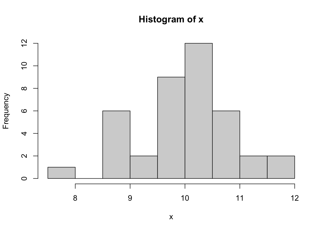

Code

boxplot(x)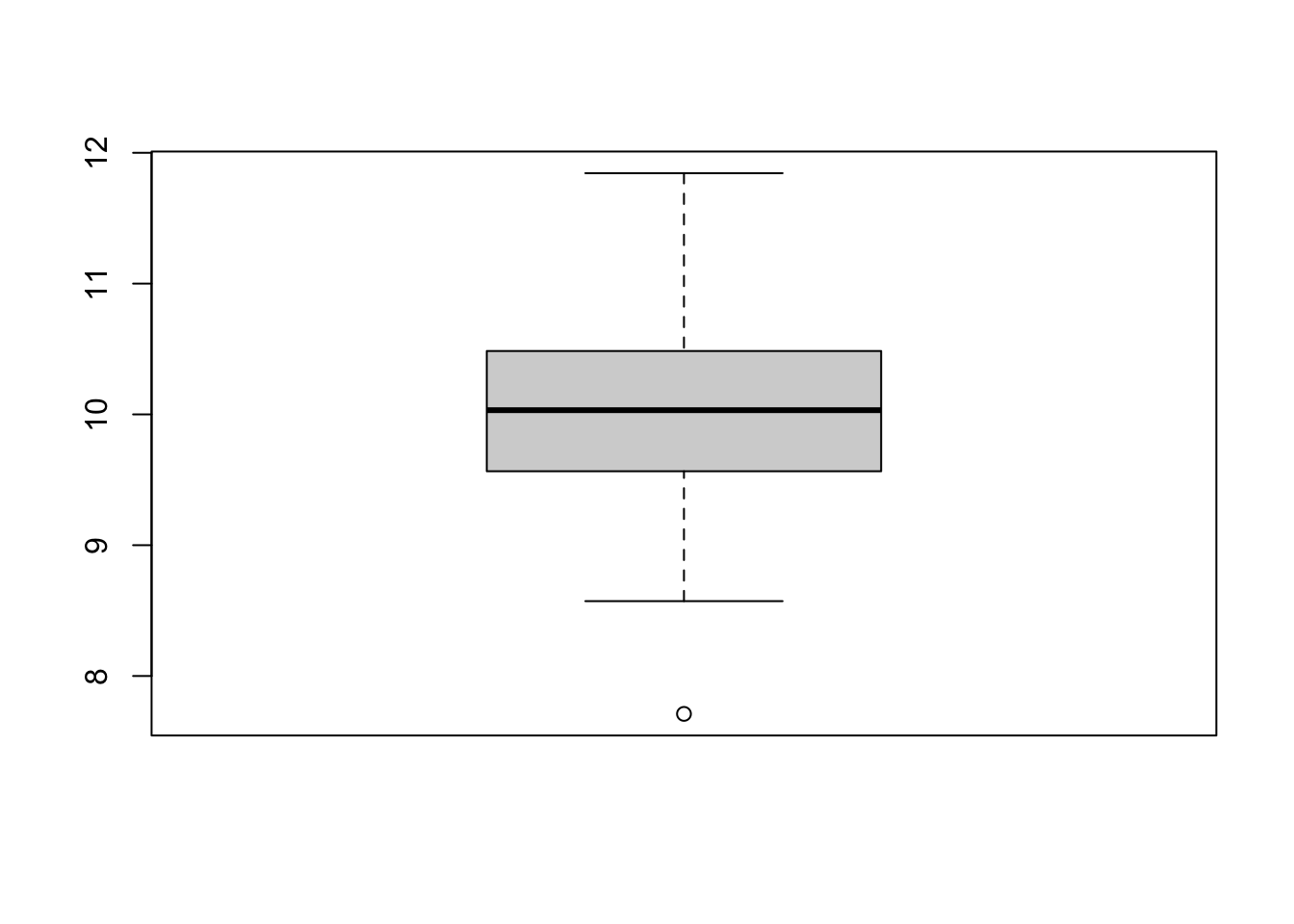

Code

plot(x)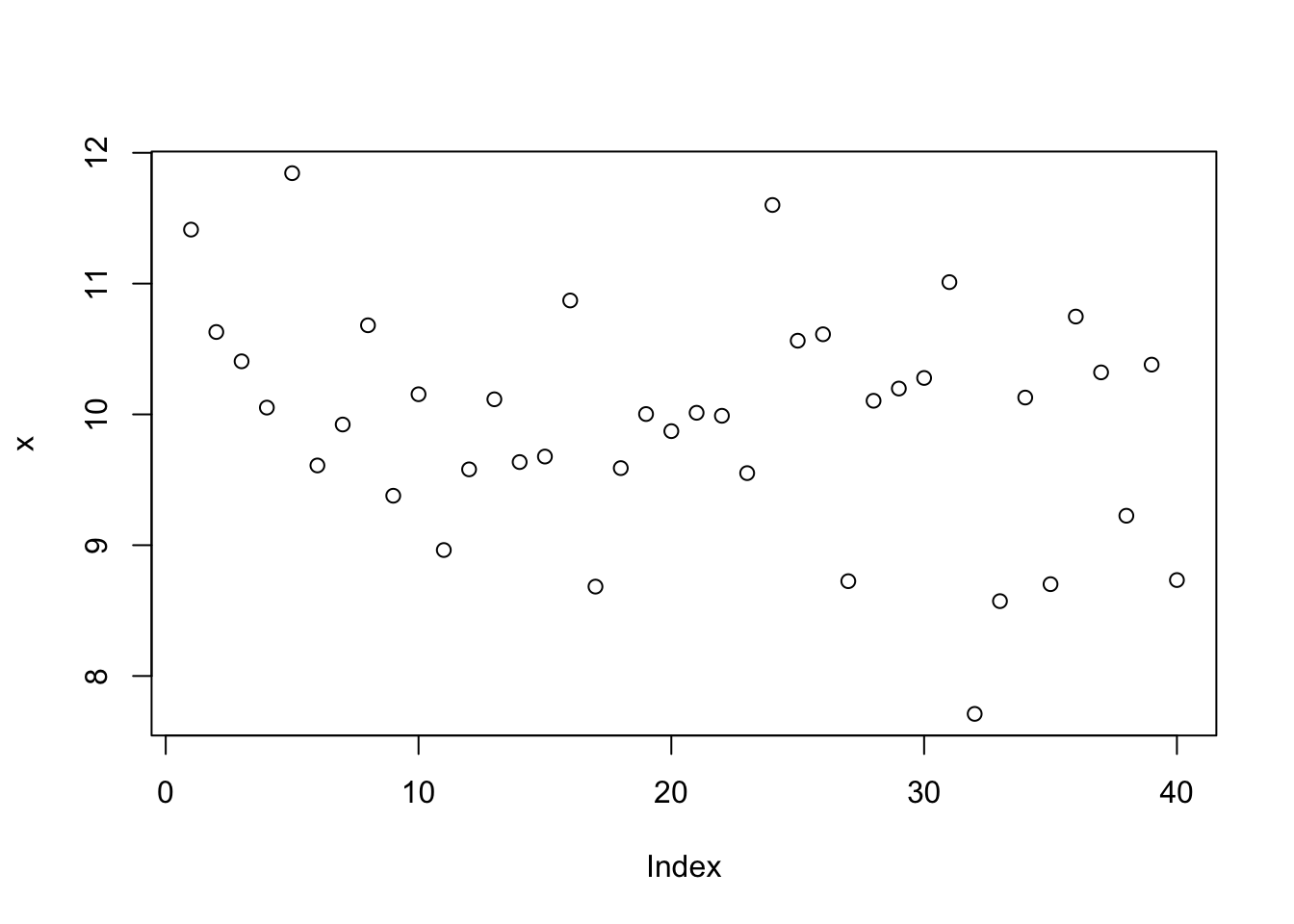

Code

plot(density(x), xlab="")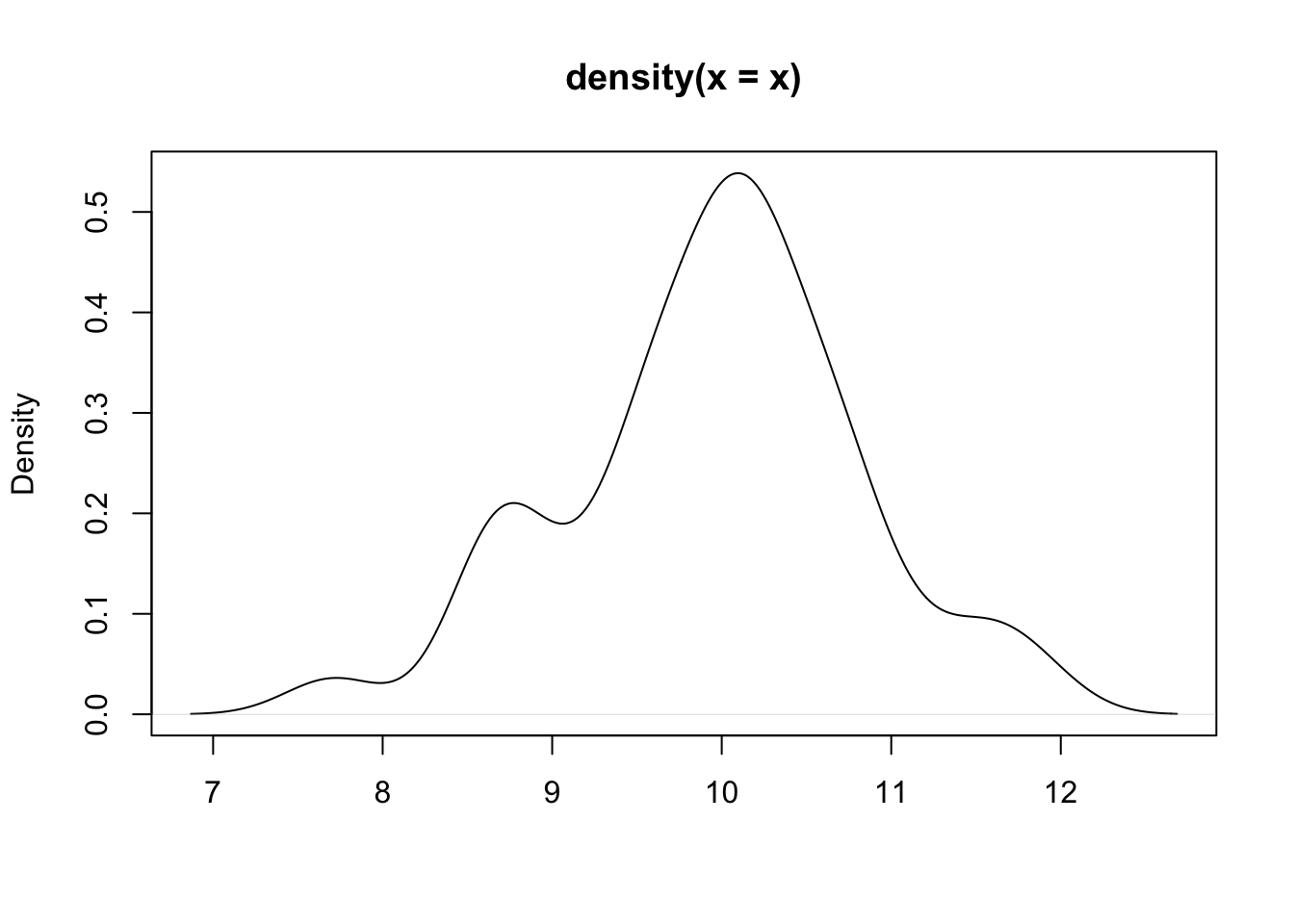

Code

stripchart(round(x,1), method = "stack", pch=20)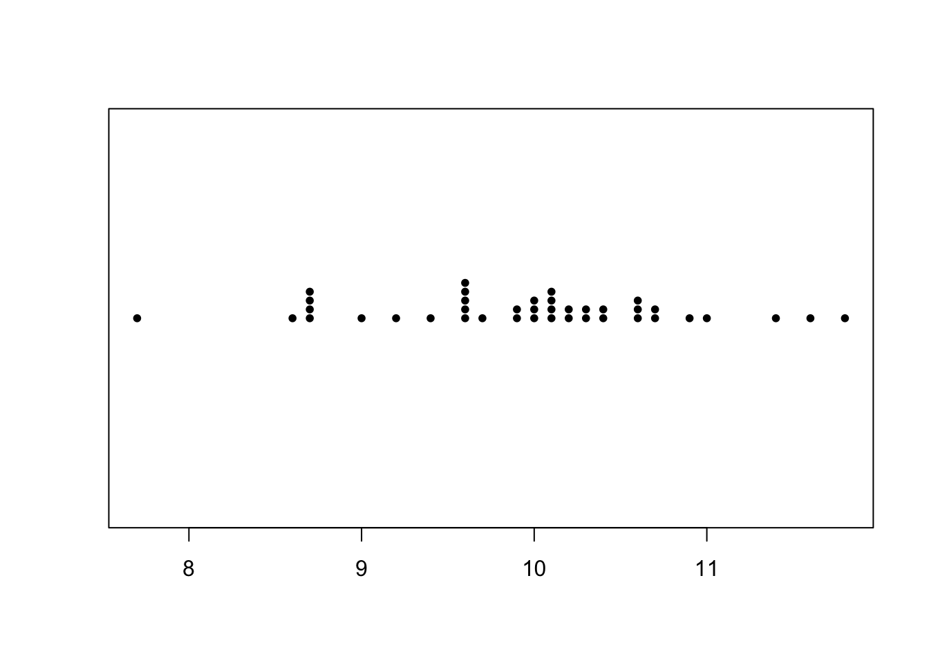

Code

plot(ecdf(x), verticals=TRUE)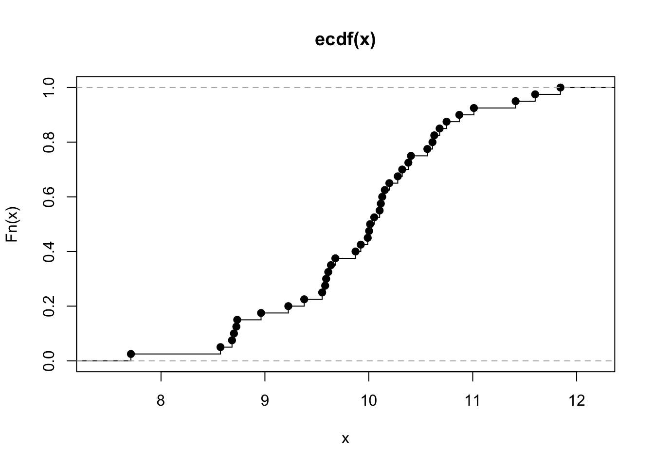

We can form a matrix of order 3X2 or (or 2X3) and display all the above six graphs in a panel. This is done using the option par(), which controls the graphics parameters.

Code

x  <- rnorm(40, 10,1)

par(mfrow = c(2, 3))

hist(x) 

boxplot(x)

plot(x)

plot(density(x), xlab='')

stripchart(round(x,1), method = "stack", pch=20)

plot(ecdf(x), verticals=TRUE)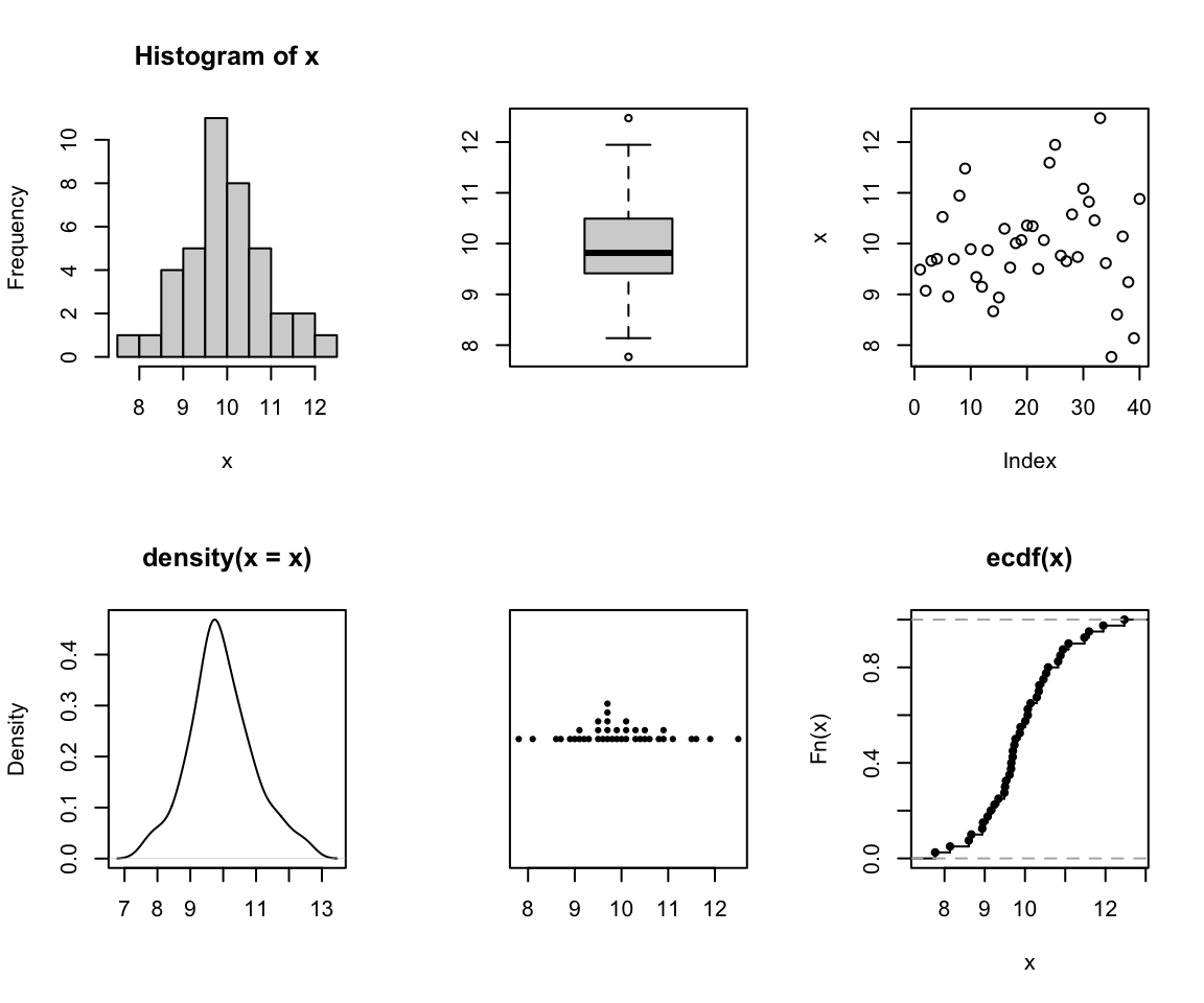

Although we shall not cover them here, many plotting options can be set using par() function; including size of margins, font types, the colour of axis labels etc. See help("par"). The option par(new=T) will be useful for an overlaid graph (instead of splitting a graph). Try the following:

Code

x  <- rnorm(40, 10,1)

plot(x, type = "o", pch = 1, ylab = "", 
     ylim = c(6.5, 13.5), lty = 1)

par(new=T)

y  <-  rnorm(40, 10,1)

plot(y, type = "o", pch = 2,
     ylab = "Two Batches of Random Normal Data",
     ylim = c(6.5, 13.5), lty = 2)

Note that pch specifies for the plotting character and lty specifies the line type. You can add a legend by the following command line:

legend("topright", c("Batch I", "Batch II"), pch=1:2, lty=1:2)

For scatter and other related plots, the command is plot(). Try

Code

x  <-  rnorm(40, 10,1)
y  <- rnorm(40, 10,1)
plot(y~x)  # or plot(x,y)

Add a title by the command

title("This is my title")

Add a reference line for the mean at the x-axis by the command

abline(v=10)

and again with abline(h=10) for the y-axis. A 45 degree (Y=X) line can be added by the command

abline(0,1) #slope, b=1, y-intercept a=1

You may also specify two points on the graph, and ask them to be connected using the command

lines(c(8, 12), c(8, 12), lty=2, col=4, lwd=2)

Note that the line() has extra arguments to control the line type, line width, and colour.

The command rug(x) draws will draw small vertical lines on the x-axis (the command actually suits better for one dimensional graphs such as a boxplot). Try

rug(x)

rug(y, side=2) #side =2 specifies y-axis

Graphs can be saved in various file formats, such as PDF (.pdf), JPEG (.jpeg or .jpg), or postscript (.ps), by enclosing the plotting function in the appropriate commands. For example, to save a simple figure as a PDF file, we use the pdf() function.

x <- 1:10

y <- x^2

pdf(file = "Fig.pdf")

plot(x, y)

dev.off()

The command dev.off() closes the file. You may use the copy and paste facility for processing graphs or use the RStudio option to save graphs.

Thelattice package contains extra graphing facilities but such graphs can be produced using ggplot2 package. Try-

Code

my.data <-read.csv(
  "https://www.massey.ac.nz/~anhsmith/data/tv.csv", 
  header=TRUE)

library(lattice)

bwplot(TELETIME ~ factor(SCHOOL), 
       data = my.data)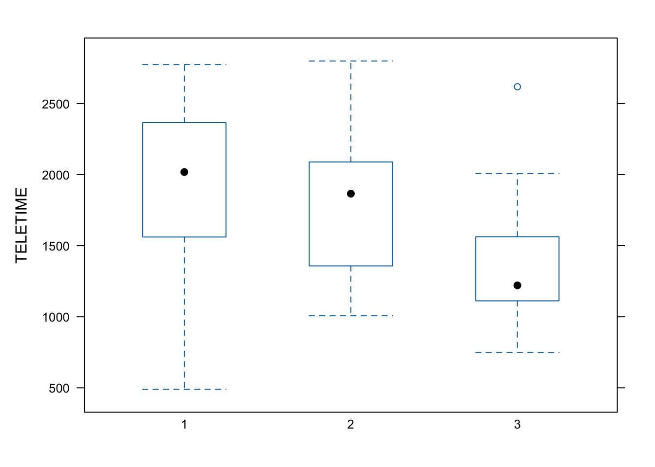

It requires a bit of coding to combine base, lattice and ggplot graphs. Try the following codes which combines three density plots of the same data produced in different styles.

Code

library("grid")
library("ggplotify")

x= rnorm(30)

p1 <- as.grob(~plot(density(x)))
p1 <- as.ggplot(p1)

p2 <- as.grob(densityplot(x))
p2 <- as.ggplot(p2)

library(ggplot2)

p3 <- data.frame(x=x) |> 
  ggplot() + 
  aes(x) +
  geom_density()

library(patchwork)

p1/(p2+p3)

Tip

It is optional to work through the activities that follow to gain an appreciation of how R works. Do not try to remember how to do everything right now. For your assignment work, we will be given the R codes to load data, graphing and modelling. These codes will give you a head-start. Note that we often often learn R by doing and sometime making mistakes.

R default options for Hypothesis tests and modelling

The stats default package in R has a number of functions for performing hypothesis tests. However you will only use the following for this course:

ks.test - Kolmogorov-Smirnov Tests

shapiro.test - Shapiro-Wilk Normality Test

t.test - Student’s t-Test (one & two samples, paired t-test etc)

pairwise.t.test - Pairwise t tests (for multiple comparison)

oneway.test - Test for Equal Means in a One-Way Layout

TukeyHSD - To Compute Tukey’s Honest Significant Differences

var.test - F Test to Compare Two Variances

bartlett.test - Bartlett Test of Homogeneity of Variances

fisher.test - Fisher’s Exact Test for Count Data

chisq.test - Pearson’s Chi-squared Test for Count Data

cor.test - Test for Association/Correlation Between Paired Samples

The car package is needed for the following:

durbinWatsonTest Durbin-Watson Test for autocorrelated Errors

leveneTest Levene’s Test

We will largely use the R function lm in this course. The syntax for specifying a model under lm command (and various other model related commands) is explained below:

The structure of the model is that the response variable is modelled as a function of the response variables. The symbol ~ (tilde) is used to say “a function of”. The simple regression of y on x is therefore specified as

lm(y ~ x)

The same applies to a one-way ANOVA in which x is a categorical factor. For example, consider tv.txt dataset and the one-way ANOVA model of TELETIME for SCHOOL is specified as follows:

Code

mydata <- read.csv(
  "https://www.massey.ac.nz/~anhsmith/data/tv.csv", 
  header=TRUE
  )

mymodel <- lm(TELETIME ~ factor(SCHOOL), 
              data = mydata) # replace lm by aov and try

summary(mymodel)

The function summary() gives the summary of the model (F statistics, residual SD etc). The model summary output can be stored into a text file using the function sink() or copy and paste in the windows version. Graphs associated with a model can be obtained using the command

plot(mymodel)

In the above context, we may also use the specific test command which will give the same result but this test can also be performed without assuming equal variances.

Code

oneway.test(TELETIME ~ SCHOOL, 
            var.equal = TRUE, 
            data = mydata)

For the lm command, note the following:

+ indicates inclusion (not addition) of an explanatory variable in the model

- indicates deletion (not subtraction) of an explanatory variable from the model

* indicates the inclusion of the explanatory variables and their interaction (not multiplication) between explanatory variables

: (colon) means only interaction between explanatory variables

/ indicates the nesting (not division) of explanatory variables

| indicates the conditioning (for example y ~ x|z means that y is a function of x for given z).

For our course, you will not use the last two types. Some model examples are given below:

lm(y ~ x + z) #regression of y on x and z (flat surface fit)

lm(y ~ x*z) #includes the interaction term ie lm(y ~ x + z + x:z)

lm(y ~ x + I(x^2) # fits a quadratic model or use poly(x,2)

lm(log(y) ~ sqrt(x) + log(z)) #all variables are transformed

As a further example, consider a study guide dataset. The following commands fit a simple regression model and then plot the fitted line on a scatter plot. Note that commands can be shortened but deliberately shown this way.

Code

mydata <- read.csv(
  "https://www.massey.ac.nz/~anhsmith/data/horsehearts.csv", 
  header=TRUE
  )

x <- mydata$EXTDIA
y <- mydata$WEIGHT

simplereg <- lm(y ~ x)

Note that our model object simplereg can be queried in many ways. The command summary() gives the following output.

Code

summary(simplereg)
# or
# library(broom)
# tidy(simplereg)
# glance(simplereg)

The command names(simplereg) will gives the names of many individual components of the object simplereg we created. For example, a plot of the residuals against the fitted values can be obtained as

Code

plot(residuals(simplereg) ~ fitted.values(simplereg))

Installing R and RStudio

Quarto

Including text and code

Setting up a Quarto project

Definitions

Introduction to the tidyverse

Tidy data

Summarize data

Group Cases

Extract cases

Alter data

Summary functions

To Use with summarize()

Further Help

R default (base) Graphing

Installing `R` and RStudio